Lab 3: Data Processing & Linear Models

This notebook is intended to get you familiar with the below topics:

• Load, explore and split data

• Using the scikit-learn library to train models (linear regression for example)

Load the real estate valuation dataset

This data set consists of the market historical data set of real estate valuation collected from Sindian Dist., Taipei City.

More on the dataset: https://archive.ics.uci.edu/dataset/477/real+estate+valuation+data+set

Load the dataset

import pandas as pd

df = pd.read_csv("./data/real_estate_valuation_dataset.csv")

Explore the data

df.head()

	No	X1 transaction date	X2 house age	X3 distance to the nearest MRT station	X4 number of convenience stores	X5 latitude	X6 longitude	Y house price of unit area
0	1	2012.916667	32.0	84.87882	10	24.98298	121.54024	37.9
1	2	2012.916667	19.5	306.59470	9	24.98034	121.53951	42.2
2	3	2013.583333	13.3	561.98450	5	24.98746	121.54391	47.3
3	4	2013.500000	13.3	561.98450	5	24.98746	121.54391	54.8
4	5	2012.833333	5.0	390.56840	5	24.97937	121.54245	43.1

len(df)

414

df["Y house price of unit area"]

0      37.9
1      42.2
2      47.3
3      54.8
4      43.1
       ... 
409    15.4
410    50.0
411    40.6
412    52.5
413    63.9
Name: Y house price of unit area, Length: 414, dtype: float64

df.describe()

	No	X1 transaction date	X2 house age	X3 distance to the nearest MRT station	X4 number of convenience stores	X5 latitude	X6 longitude	Y house price of unit area
count	414.000000	414.000000	414.000000	414.000000	414.000000	414.000000	414.000000	414.000000
mean	207.500000	2013.148953	17.712560	1083.885689	4.094203	24.969030	121.533361	37.980193
std	119.655756	0.281995	11.392485	1262.109595	2.945562	0.012410	0.015347	13.606488
min	1.000000	2012.666667	0.000000	23.382840	0.000000	24.932070	121.473530	7.600000
25%	104.250000	2012.916667	9.025000	289.324800	1.000000	24.963000	121.528085	27.700000
50%	207.500000	2013.166667	16.100000	492.231300	4.000000	24.971100	121.538630	38.450000
75%	310.750000	2013.416667	28.150000	1454.279000	6.000000	24.977455	121.543305	46.600000
max	414.000000	2013.583333	43.800000	6488.021000	10.000000	25.014590	121.566270	117.500000

import matplotlib.pyplot as plt


def plot_histogram(data):
    fig, ax = plt.subplots()
    ax.hist(data, bins=20)
    ax.set_xlabel("Value")
    ax.set_ylabel("Frequency")

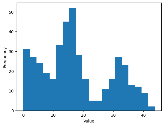
plot_histogram(df["X2 house age"])

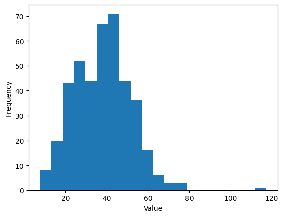
plot_histogram(df["Y house price of unit area"])

def plot_scatter(X, Y):
    fig, ax = plt.subplots()
    ax.scatter(X, Y)
    ax.set_xlabel("Horizonal")
    ax.set_ylabel("Vertical")

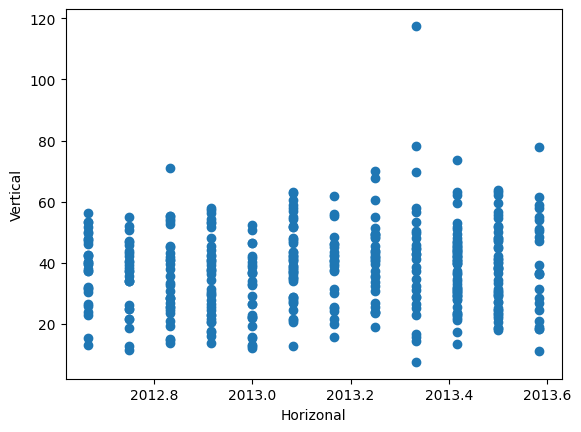
plot_scatter(df["X1 transaction date"], df["Y house price of unit area"])

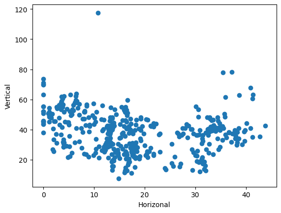
plot_scatter(df["X2 house age"], df["Y house price of unit area"])

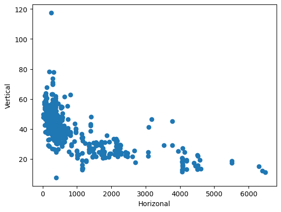
plot_scatter(
    df["X3 distance to the nearest MRT station"], df["Y house price of unit area"]
)

Convert to other formats

Y = df["Y house price of unit area"]
type(Y)

pandas.core.series.Series

Y1 = Y.to_list()
type(Y1)

list

Y2 = Y.to_numpy()
type(Y2)

numpy.ndarray

# save as an excel xlsx file

df.to_excel("./data/real_estate_valuation_dataset.xlsx", index=False)

Split dataset

Convert to numpy arrays

features = [
    "X1 transaction date",
    "X2 house age",
    "X3 distance to the nearest MRT station",
    "X4 number of convenience stores",
    "X5 latitude",
    "X6 longitude",
]
X = df[features].to_numpy()

X.shape

(414, 6)

type(X)

numpy.ndarray

y = df["Y house price of unit area"].to_numpy()

y.shape

(414,)

type(y)

numpy.ndarray

from sklearn.model_selection import train_test_split

Split by ratio

X_train, X_test, y_train, y_test = train_test_split(X, y, test_size=0.2, random_state=0)

print("X_train.shape =", X_train.shape)
print("X_test.shape =", X_test.shape)

X_train.shape = (331, 6)
X_test.shape = (83, 6)

Split by number

X_train, X_test, y_train, y_test = train_test_split(X, y, test_size=100, random_state=0)

print("X_train.shape =", X_train.shape)
print("X_test.shape =", X_test.shape)

X_train.shape = (314, 6)
X_test.shape = (100, 6)

Use random seed to make it reproducible

X_train, X_test, y_train, y_test = train_test_split(X, y, test_size=100)

X_train[0]

array([2013.4166667,    4.3      ,  432.0385   ,    7.       ,
         24.9805   ,  121.53778  ])

Train, validation, test split

X_dev, X_test, y_dev, y_test = train_test_split(X, y, test_size=0.1, random_state=0)
X_train, X_val, y_train, y_val = train_test_split(
    X_dev, y_dev, test_size=0.1, random_state=1
)

print("X_train.shape =", X_train.shape)
print("X_val.shape =", X_val.shape)
print("X_test.shape =", X_test.shape)

X_train.shape = (334, 6)
X_val.shape = (38, 6)
X_test.shape = (42, 6)

Fit linear model

Linear regression

from sklearn.linear_model import LinearRegression
from sklearn.metrics import mean_squared_error

model = LinearRegression()
model.fit(X_train, y_train)

LinearRegression()

In a Jupyter environment, please rerun this cell to show the HTML representation or trust the notebook.
On GitHub, the HTML representation is unable to render, please try loading this page with nbviewer.org.

y_pred = model.predict(X_train)
mae = mean_squared_error(y_train, y_pred)

print("MSE on training set =", mae)

MSE on training set = 82.4146645368272

y_pred = model.predict(X_test)
mae = mean_squared_error(y_test, y_pred)

print("MSE on test set =", mae)

MSE on test set = 51.83750374286789

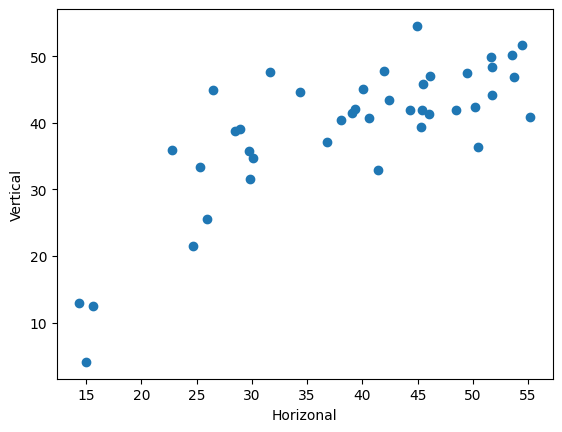
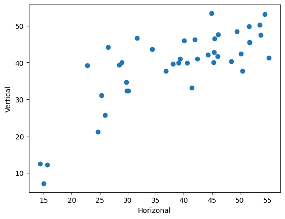
plot_scatter(y_test, y_pred)

Cross validation

Q: What is the effect of data splitting on the model performance?

from sklearn.model_selection import cross_validate

model = LinearRegression()
cv_results = cross_validate(
    model, X, y, cv=5, scoring="neg_mean_squared_error", return_train_score=True
)

cv_results["test_score"]

array([ -49.89284058,  -89.03269132,  -57.8698601 , -134.81795278,
        -60.0483656 ])

Ridge regression

Q: What is the effect of regularization on the model performance?

from sklearn.linear_model import Ridge

model = Ridge(alpha=0.1)
model.fit(X_train, y_train)
y_pred = model.predict(X_test)

mean_squared_error(y_test, y_pred)

55.2204325346256

plot_scatter(y_test, y_pred)